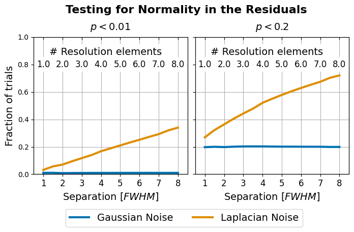
Figure 14: Shapiro-Wilk test#
This code is used to create Figure 14 in the Apples with Apples paper (Bonse et al. 2023). The Figure shows the sensitivity of the Shapiro-Wilk test as a function of separation from the star. We study two cases: 1. The false positive fraction of the Shapiro-Wilk test in case of Gaussian noise. 2. The sensitivity i.e. true positive fractionof the Shapiro-Wilk in case of Laplactian noise.
Imports#
[1]:
import os
import random
import pickle
import numpy as np
from scipy import stats
from tqdm import tqdm
import seaborn as sns

import matplotlib.pyplot as plt

from applefy.utils.mc_simulations import draw_mc_sample
from applefy.utils.file_handling import read_apples_with_apples_root
Monte-Carlo Simulation#
First we need to run the monte carlo simulation. This step is computationally very expensive. If you just want to reproduce the plot you can skip this part and restore the results from Zenodo.
[2]:
# Compute the number of independent resolution elements
separations = np.linspace(1, 8, 15)
num_res_elements = [(int(np.floor(np.pi*2*i)), i) for i in separations]
Run the actual monte-carlo simulation.
[3]:
np.random.seed(42)
num_tests= 1e6

p_values_normal = dict()
p_values_laplace = dict()

for tmp_num_res, tmp_separation in num_res_elements:
    print("Running separation " + str(tmp_separation))

    # Draw noise
    _, res_values_normal, _ = draw_mc_sample(
        tmp_num_res,
        num_draws=num_tests,
        noise_distribution="gaussian",
        num_cores=32,
        loc_noise=1,
        scale_noise=1)

    _, res_values_laplace, _ = draw_mc_sample(
        tmp_num_res,
        num_draws=num_tests,
        noise_distribution="laplace",
        num_cores=32,
        loc_noise=1,
        scale_noise=1)

    # Compute p-values
    p_values_normal[tmp_separation] = []
    p_values_laplace[tmp_separation] = []

    for i in tqdm(range(int(num_tests))):
        p_values_normal[tmp_separation].append(
            stats.shapiro(res_values_normal[i, :]).pvalue)
        p_values_laplace[tmp_separation].append(
            stats.shapiro(res_values_laplace[i, :]).pvalue)
Running separation 1.0
100%|██████████████████████████████████████████████████████████████████████████████████████████████████████████████████████████████████████████████████████████| 1000000/1000000 [01:08<00:00, 14681.50it/s]
Running separation 1.5
100%|██████████████████████████████████████████████████████████████████████████████████████████████████████████████████████████████████████████████████████████| 1000000/1000000 [01:08<00:00, 14605.14it/s]
Running separation 2.0
100%|██████████████████████████████████████████████████████████████████████████████████████████████████████████████████████████████████████████████████████████| 1000000/1000000 [01:09<00:00, 14298.64it/s]
Running separation 2.5
100%|██████████████████████████████████████████████████████████████████████████████████████████████████████████████████████████████████████████████████████████| 1000000/1000000 [01:09<00:00, 14456.29it/s]
Running separation 3.0
100%|██████████████████████████████████████████████████████████████████████████████████████████████████████████████████████████████████████████████████████████| 1000000/1000000 [01:06<00:00, 15059.11it/s]
Running separation 3.5
100%|██████████████████████████████████████████████████████████████████████████████████████████████████████████████████████████████████████████████████████████| 1000000/1000000 [01:08<00:00, 14615.66it/s]
Running separation 4.0
100%|██████████████████████████████████████████████████████████████████████████████████████████████████████████████████████████████████████████████████████████| 1000000/1000000 [01:08<00:00, 14507.22it/s]
Running separation 4.5
100%|██████████████████████████████████████████████████████████████████████████████████████████████████████████████████████████████████████████████████████████| 1000000/1000000 [01:09<00:00, 14337.79it/s]
Running separation 5.0
100%|██████████████████████████████████████████████████████████████████████████████████████████████████████████████████████████████████████████████████████████| 1000000/1000000 [01:08<00:00, 14642.79it/s]
Running separation 5.5
100%|██████████████████████████████████████████████████████████████████████████████████████████████████████████████████████████████████████████████████████████| 1000000/1000000 [01:08<00:00, 14550.62it/s]
Running separation 6.0
100%|██████████████████████████████████████████████████████████████████████████████████████████████████████████████████████████████████████████████████████████| 1000000/1000000 [01:10<00:00, 14091.97it/s]
Running separation 6.5
100%|██████████████████████████████████████████████████████████████████████████████████████████████████████████████████████████████████████████████████████████| 1000000/1000000 [01:08<00:00, 14502.08it/s]
Running separation 7.0
100%|██████████████████████████████████████████████████████████████████████████████████████████████████████████████████████████████████████████████████████████| 1000000/1000000 [01:11<00:00, 14012.24it/s]
Running separation 7.5
100%|██████████████████████████████████████████████████████████████████████████████████████████████████████████████████████████████████████████████████████████| 1000000/1000000 [01:10<00:00, 14105.61it/s]
Running separation 8.0
100%|██████████████████████████████████████████████████████████████████████████████████████████████████████████████████████████████████████████████████████████| 1000000/1000000 [01:10<00:00, 14153.04it/s]
Save the results.
[4]:
result_dir = os.path.join(
    read_apples_with_apples_root(),
    "70_results/shapiro_wilk_tests/")
Data in the APPLES_ROOT_DIR found. Location: /home/ipa/quanz/user_accounts/mbonse/2021_Metrics/70_results/apples_root_dir
[5]:
# Save as .pkl
with open(os.path.join(result_dir, 'A1_Shapiro_normal.pkl'), 'wb') as handle:
    pickle.dump(p_values_normal, handle, protocol=pickle.HIGHEST_PROTOCOL)

with open(os.path.join(result_dir, 'A1_Shapiro_laplace.pkl'), 'wb') as handle:
    pickle.dump(p_values_laplace, handle, protocol=pickle.HIGHEST_PROTOCOL)
Alternative: restore the results#
Restore the results of the Monte-Carlo simulation. In order to run the code make sure to download the data from Zenodo andread the instructionson how to setup the files.
[6]:
result_dir = os.path.join(
    read_apples_with_apples_root(),
    "70_results/shapiro_wilk_tests/")
Data in the APPLES_ROOT_DIR found. Location: /home/ipa/quanz/user_accounts/mbonse/2021_Metrics/70_results/apples_root_dir
The restored results just contain the p-values of the test for Gaussian noise (false positives) and Laplacian noise (true positives).
[7]:
# Load .pkl
with open(os.path.join(result_dir, 'A1_Shapiro_normal.pkl'), 'rb') as handle:
    p_values_normal = pickle.load(handle)

with open(os.path.join(result_dir, 'A1_Shapiro_laplace.pkl'), 'rb') as handle:
    p_values_laplace = pickle.load(handle)
Compute FPF and TPF#
We compute the false positive fraction (FPF) and true positive fraction (TPF) for two different confidence levels: \(p<0.01\) and \(p<0.2\).
[8]:
# FPF
normal_p_001 = [np.sum(np.array(p_values) < 0.01) /
                len(p_values) for p_values in p_values_normal.values()]
# TPF
laplace_p_001 = [np.sum(np.array(p_values) < 0.01) / len(p_values)
                 for p_values in p_values_laplace.values()]

# FPF
normal_p_02 = [np.sum(np.array(p_values) < 0.2) / len(p_values)
               for p_values in p_values_normal.values()]
# TPF
laplace_p_02 = [np.sum(np.array(p_values) < 0.2) / len(p_values)
                for p_values in p_values_laplace.values()]
Make the Plot#
Define the colors we want to use for the plot.
[9]:
color_palette = [sns.color_palette("colorblind")[0],
                 sns.color_palette("colorblind")[1]]
A small function to plot the two cases \(p<0.01\) and \(p<0.2\).
[10]:
def plot_results(
    axis_in,
    fpf_values,
    tpf_values,
    title):

    # Plot the fpf and tpf
    axis_in.plot(
        p_values_normal.keys(),
        fpf_values,
        lw=3, color=color_palette[0],
        label="Gaussian Noise")

    axis_in.plot(
        p_values_normal.keys(),
        tpf_values,
        lw=3, color=color_palette[1],
        label="Laplacian Noise")

    axis_in.grid()
    axis_in.set_ylim(0, 1)
    axis_in.set_xlim(0.5, 8.5)
    axis_in.set_xticks(np.arange(1,9))

    # Change the Labels and ticks
    for tick in axis_in.xaxis.get_major_ticks():
        tick.label1.set_fontsize(12)

    # second x axis for the number of Resolution elements
    axis_in_2 = axis_in.twiny()

    axis_in_2.set_xticks(np.arange(1, 9))
    axis_in_2.tick_params(axis="x",direction="in", pad=-45)

    axis_in_2.set_xticklabels(
        [i[1] for i in num_res_elements][::2], fontsize=12)
    axis_in_2.set_xlim(0.5, 8.5)

    for tmp_label in axis_in_2.xaxis.get_ticklabels():
        tmp_label.set_bbox(dict(facecolor='white', edgecolor='none'))

    axis_in_2.text(
        1.3, 0.87, "# Resolution elements",
        bbox=dict(facecolor='white', edgecolor='none'),
        fontsize=14)

    axis_in.set_title(title, fontsize=14, y=1.02)
    axis_in.set_xlabel(r"Separation $[FWHM]$", fontsize=14)
Create the actual plot.
[11]:
# 1.) Create the Figure Layout
fig = plt.figure(constrained_layout=False,
                 figsize=(8, 3.5))

gs0 = fig.add_gridspec(1, 2)
gs0.update(hspace=0.1, wspace=0.05)

low = fig.add_subplot(gs0[0, 0])
high = fig.add_subplot(gs0[0, 1],
                       sharey=low, sharex=low)

# 2.) Plot 1: p < 0.01
plot_results(
    axis_in=low,
    fpf_values=normal_p_001,
    tpf_values=laplace_p_001,
    title=r"$p < 0.01$")
low.set_ylabel("Fraction of trials", fontsize=14)

# 3.) Plot 2: p < 0.2
plot_results(
    axis_in=high,
    fpf_values=normal_p_02,
    tpf_values=laplace_p_02,
    title=r"$p < 0.2$")

plt.setp(high.get_yticklabels(), visible=False)

# 4.) Legend
lgd = low.legend(loc='center right',ncol=2,
                 bbox_to_anchor=(1.78, -0.32),
                 fontsize=14,
                 markerscale=3.,)

fig_title = fig.suptitle(
    "Testing for Normality in the Residuals",
    size=16, fontweight="bold", y=1.06)

fig.patch.set_facecolor('white')
plt.savefig("./14_Residual_Shapiro.pdf",
            bbox_extra_artists=(lgd, fig_title),
            bbox_inches='tight')