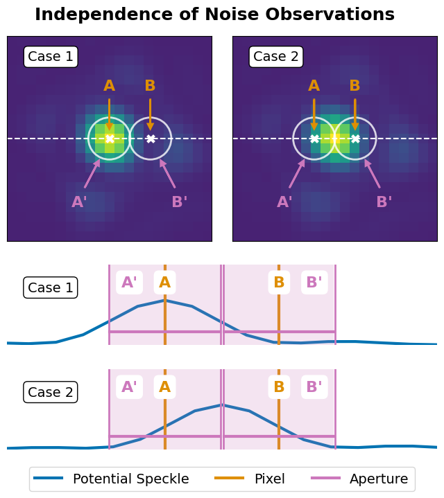
Figure 2: Independence#
This is the code used to create Figure 2 in the Apples with Apples paper (Bonse et al. 2023). The code illustrates how the use of apertures violates the independence assumption of the T-test.
Imports#
[1]:
import os
import json
from pathlib import Path
import numpy as np
import matplotlib.pyplot as plt
import matplotlib.gridspec as gridspec
import seaborn as sns

from applefy.utils.file_handling import read_apples_with_apples_root, \
    open_fits, load_adi_data
from applefy.gaussianity.residual_tests import extract_circular_annulus
Data Loading#
To illustrate the size of the speckles we load the unsaturated PSF. In order to run the code make sure to download the data from Zenodo andread the instructionson how to setup the files.
[2]:
experiment_root = read_apples_with_apples_root()
Data in the APPLES_ROOT_DIR found. Location: /home/ipa/quanz/user_accounts/mbonse/2021_Metrics/70_results/apples_root_dir
[3]:
dataset_file = experiment_root / Path("30_data/betapic_naco_lp_LR.hdf5")
science_data_key = "science_no_planet"
psf_template_key = "psf_template"
parang_key = "header_science_no_planet/PARANG"

dit_psf_template = 0.02019
dit_science = 0.2
fwhm = 4.2  # estimeated with Pynpoint in advance
[4]:
# we need the psf template for contrast calculation
_, _, raw_psf_template_data = load_adi_data(
    dataset_file,
    data_tag=science_data_key,
    psf_template_tag=psf_template_key,
    para_tag=parang_key)
The unsaturated PSF template is very large, we crop it to 21 x 21 pixel.
[5]:
psf_template_data = raw_psf_template_data[82:-82, 82:-82]
Create the plot#
This is a small helper function which is used to label the images of the PSF.
[6]:
def plot_psf_with_positions(positions_in,
                            axis_in,
                            case_label):

    # Show the PSF
    axis_in.imshow(psf_template_data,
                   vmin=-np.max(psf_template_data)*0.1,
                   vmax=np.max(psf_template_data))

    axis_in.text(4, 2, case_label, ha="center", color="black",
                 bbox=dict(facecolor='white',
                           boxstyle="round",
                           edgecolor="black"),
                 fontsize=14)


    # Plot the Positions of the Apertures and pixel
    axis_in.scatter(positions_in[0],
                    positions_in[1],
                    marker="o", s=1900,
                    edgecolor="white",
                    lw=2, facecolor="None",
                    alpha=0.8)

    axis_in.scatter(positions_in[0],
                    positions_in[1],
                    marker="x", s=50,
                    color="white",
                    lw=3,
                    alpha=1)

    # Write Names of the Positions (Pixel)
    axis_in.text(positions_in[0][0],
                 positions_in[1][0] - 5, "A",
                 fontsize=16, fontweight="bold", ha="center",
                 color=sns.color_palette("colorblind")[1])

    axis_in.text(positions_in[0][1],
                 positions_in[1][1] - 5, "B",
                 fontsize=16, fontweight="bold",  ha="center",
                 color=sns.color_palette("colorblind")[1])

    axis_in.arrow(positions_in[0][0],
                  positions_in[1][0] - 4,
                  0, 2.5, lw=2,
                  head_width=0.5, head_length=0.5,
                  color=sns.color_palette("colorblind")[1])

    axis_in.arrow(positions_in[0][1],
                  positions_in[1][1] - 4,
                  0, 2.5, lw=2,
                  head_width=0.5, head_length=0.5,
                  color=sns.color_palette("colorblind")[1])

    # Write Names of the Positions (Apertures)
    axis_in.text(positions_in[0][0] - 3,
                 positions_in[1][0] + 7, "A'",
                 fontsize=16, fontweight="bold", ha="center",
                 color=sns.color_palette("colorblind")[4])

    axis_in.arrow(positions_in[0][0] - 2.5,
                  positions_in[1][0] + 5,
                  1.2, -2.3, lw=2,
                  head_width=0.5, head_length=0.5,
                  color=sns.color_palette("colorblind")[4])

    axis_in.text(positions_in[0][1] + 3,
                 positions_in[1][1] + 7, "B'",
                 fontsize=16, fontweight="bold", ha="center",
                 color=sns.color_palette("colorblind")[4])

    axis_in.arrow(positions_in[0][1] + 2.5,
                  positions_in[1][1] + 5,
                  -1.2, -2.3, lw=2,
                  head_width=0.5, head_length=0.5,
                  color=sns.color_palette("colorblind")[4])


    # Remove the axis
    axis_in.axes.get_xaxis().set_ticks([])
    axis_in.axes.get_yaxis().set_ticks([])

    # Plot the horizontal line to mark the cut below
    axis_in.axhline(psf_template_data.shape[0]/2 - 0.5,
                    color="white", ls="--")
This is a small helper function which is used to create the sketches for Case 1 and Case 2.
[8]:
psf_line = psf_template_data[:,10] - np.min(psf_template_data[:,10])
psf_line /= np.max(psf_line)

def plot_illustration(pos_A,
                      pos_B,
                      shift,
                      axis_in):

    axis_in.plot(psf_line,
                 lw=3,label="Potential Speckle",
                 color = sns.color_palette("colorblind")[0])

    axis_in.set_xlim(2.1 + shift, len(psf_line) - 3.1 + shift)
    axis_in.set_ylim(0, 1.8)
    axis_in.axvline(pos_A, lw=3,
                    color=sns.color_palette("colorblind")[1],
                    label="Pixel",)
    axis_in.axvline(pos_B, lw=3,
                    color=sns.color_palette("colorblind")[1])

    axis_in.axvline(pos_A, lw=114,
                    color=sns.color_palette("colorblind")[4], alpha=0.2)
    axis_in.axvline(pos_B, lw=114,
                    color=sns.color_palette("colorblind")[4], alpha=0.2)

    # Aperture area
    line = plt.Line2D(
        (pos_A - 2.03, pos_A + 2.03),
        (0.3, 0.3), lw=3, mew=3,
        color=sns.color_palette("colorblind")[4])#,
        #marker="|", ms=10)

    axis_in.add_line(line)
    axis_in.axvline(pos_A - 2.05, lw=2,
                    color=sns.color_palette("colorblind")[4])
    axis_in.axvline(pos_A + 2.05, lw=2,
                    color=sns.color_palette("colorblind")[4])

    line = plt.Line2D(
        (pos_B - 2.03, pos_B + 2.03),
        (0.3, 0.3), lw=3, mew=3, label="Aperture",
        color=sns.color_palette("colorblind")[4])#,
        #marker="|", ms=10)

    axis_in.add_line(line)

    axis_in.axvline(pos_B - 2.05, lw=2,
                    color=sns.color_palette("colorblind")[4])
    axis_in.axvline(pos_B + 2.05, lw=2,
                    color=sns.color_palette("colorblind")[4])

    # Add all labels
    axis_in.text(pos_A, 1.4, "A",
                 ha="center", size=16,
                 color=sns.color_palette("colorblind")[1],
                 va="center", fontweight="bold",
                 bbox=dict(facecolor='white',
                           boxstyle="round",
                           edgecolor="white"))

    axis_in.text(pos_A - 1.3, 1.4, "A'",
                 ha="center", size=16,
                 color=sns.color_palette("colorblind")[4],
                 va="center", fontweight="bold",
                 bbox=dict(facecolor='white',
                           boxstyle="round",
                           edgecolor="white"))

    axis_in.text(pos_B, 1.4, "B",
                 ha="center", size=16,
                 color=sns.color_palette("colorblind")[1],
                 va="center", fontweight="bold",
                 bbox=dict(facecolor='white',
                           boxstyle="round",
                           edgecolor="white"))

    axis_in.text(pos_B + 1.3, 1.4, "B'",
                 ha="center", size=16,
                 color=sns.color_palette("colorblind")[4],
                 va="center", fontweight="bold",
                 bbox=dict(facecolor='white',
                           boxstyle="round",
                           edgecolor="white"))

    axis_in.axis("off")
Create the final plot.
[9]:
# 1.) Make the plot gridlayout
fig = plt.figure(constrained_layout=False,
                 figsize=(8, 8))
gs0 = fig.add_gridspec(2, 1, height_ratios=[2.5, 2])
gs0.update(hspace=0.05, wspace=0.15)

gs1 = gridspec.GridSpecFromSubplotSpec(1, 2,
                                       subplot_spec=gs0[0],
                                       hspace=0., wspace=0.1,
                                       width_ratios=[1, 1])

gs2 = gridspec.GridSpecFromSubplotSpec(2, 1,
                                       subplot_spec=gs0[1],
                                       hspace=0.3, wspace=0.1,
                                       height_ratios=[1, 1])

ax_psf_case1 = fig.add_subplot(gs1[0])
ax_psf_case2 = fig.add_subplot(gs1[1])
ax_illustration1 = fig.add_subplot(gs2[0])
ax_illustration2 = fig.add_subplot(gs2[1])


# 2.) Plot the unsaturated PSF with apertures on top of it
plot_psf_with_positions(([10, 10 + 4.2], [10,10],),
                        ax_psf_case1, "Case 1")
plot_psf_with_positions(([10 - 2.1, 10 + 2.1], [10,10],),
                        ax_psf_case2, "Case 2")

# 3.) Plot the illustrations for Case 1 and Case 2
plot_illustration(10, 10 + 4.2, 2.1,  ax_illustration1)
plot_illustration(10 - 2.1, 10 + 2.1, 0, ax_illustration2)

plt.setp(ax_illustration1.get_xticklabels(), visible=False)

ax_illustration1.text(3.7 + 2.1, 1.2, "Case 1", ha="center", color="black",
                      fontsize=14, #fontweight="bold",
                      bbox=dict(facecolor='white',
                                boxstyle="round",
                                edgecolor="black"))

ax_illustration2.text(3.7, 1.2, "Case 2", ha="center", color="black",
                     fontsize=14, #fontweight="bold",
                     bbox=dict(facecolor='white',
                               boxstyle="round",
                               edgecolor="black"))

# 4.) Add a legend
lgd = ax_illustration2.legend(ncol=3, fontsize=14,
                              loc='lower center',
                              bbox_to_anchor=(0.5, -0.6))

st = fig.suptitle("Independence of Noise Observations",
                  fontsize=18, fontweight="bold", y=0.91)

# 5.) Save the figure
fig.patch.set_facecolor('white')
plt.savefig("./02_Independence.pdf",
            bbox_extra_artists=(lgd, st),
            bbox_inches='tight')